
Machine Vision PID Control
For the final project in my Dynamics & Control System Design laboratory course, I was tasked with controlling the position of a ping pong ball in a clear tube using a simple DC cooling fan. This project utilized PID control, bilinear mapping, and machine vision to achieve the desired system performance. Full report link here.
Background
Given the objective of controlling the position of the ping pong ball within the tube, a simplified free body diagram was created to understand the forces acting on the ball. The system was idealized to show the ball in free fall, where its only contributing forces were the force of gravity and the drag force. At a critical fan velocity, the drag force would cancel with the force of gravity, which would result in the ball floating in space. Given the linear relationship between fan speed and input voltage, a feedforward voltage was determined to create a force balance between the two free fall forces. From there, any input voltage above or below the feedforward term would cause the ball to accelerate upwards or downwards respectively.

Experimental Setup
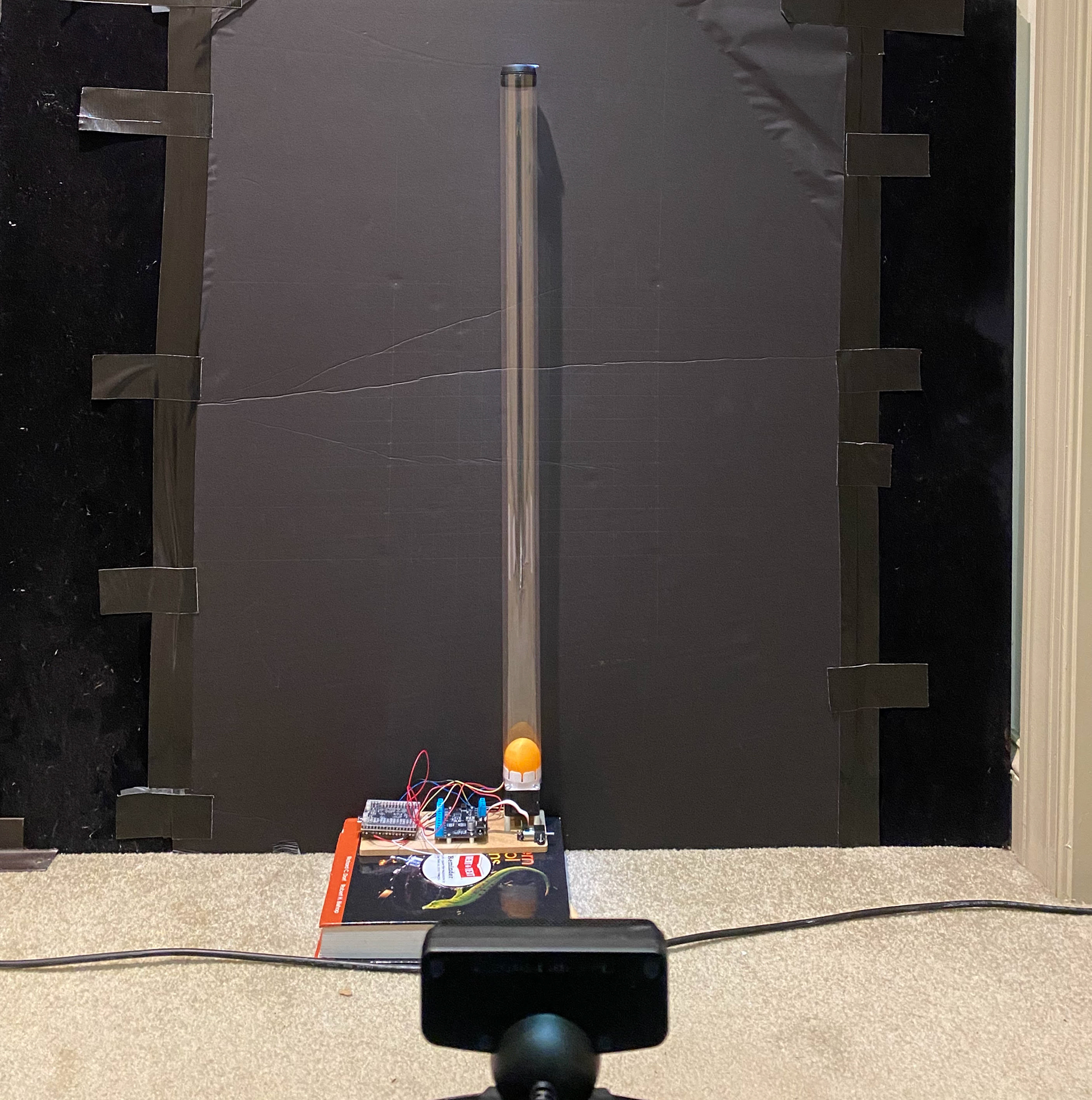
The plant consisted of a 41.5 mm diameter polycarbonate tube (53 cm length), a 40 mm diameter orange ping pong ball, a 12V DC brushless cooling fan and a 3D-printed fan-tube connection hub. The fan was wired to a SADI 2.2 data acquisition device (DAQ) and a SADI motor controller. The DAQ was connected to LabVIEW, and the motor controller was connected to a 12V power supply. The plant was positioned behind a dark background with ambient lighting to help the Playstation 3 Eye camera threshold the position of the ball.
Bilinear Mapping
Given that the camera could not be perfectly aligned with the plant, a process call bilinear mapping was implemented to record the ball’s position in pixel space and convert that position to its respective world space

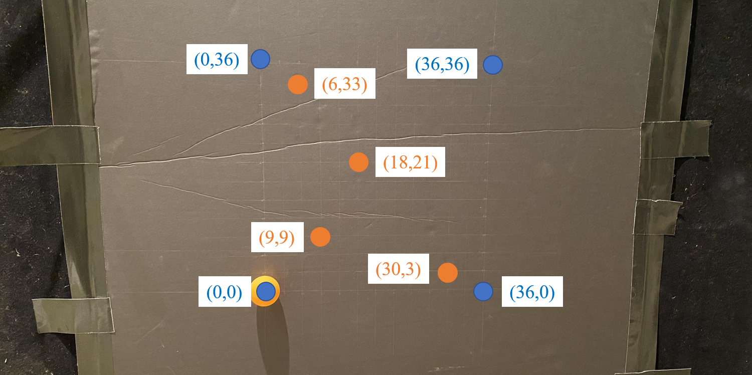
Bilinear mapping accounts for the misalignment of the camera and the plant by taking four points in the plant’s background and their known world coordinates (measured with a ruler) and linearly relating those world coordinates to the respective pixel coordinates. To facilitate this process, a 36 cm x 36 cm square grid was drawn onto the background poster board to determine calibration (blue) and test (orange) points.
The linear relationship between the world space and pixel space coordinates is defined below, where the "c" terms correspond to the linear coefficients needed to solve the system

By rearranging the two equations above in matrix format, the coefficients can be calculated by taking the inverse of the pixel matrix and multiplying it by the world space vector. To simplify this calculation, a MATLAB script was created and used to solve for the calibration coefficients.


LabVIEW Virtual Instrument (VI)
A virtual instrument was created to send feedback commands to the motor controller. The VI (shown below) consists of two while loops, where the upper loop iterates as a function of the DAQ sampling rate, and the lower loop iterates as a function of the PS3 camera sampling rate. Key elements of the VI are described below. The calibration coefficients calculated from the MATLAB script above were input into the upper loop to calculate the real-time position of the ball.

The desired trajectory of the ball was created using the subVI listed below, where three different heights were selected for the ball to track. For the ball to move on to the next desired trajectory value, the ball's thresholded centroid location would need to be within a preset error tolerance for a preset amount of time.

Error in the system was determined by taking the difference in the desired height and the real-time position of the ball (wy). The system error was used to fuel the PID controller, where the error and its respective derivative and integral were used as input terms in the controller.

To reduce noise in the system, point-by-point mean filters were added to the pixel X & Y position variables before computing the real-time position. The pixel coordinates fluctuated due to noise from the lighting setup, so the oscillations were reduced by average the recorded values over 100 points. Similarly, a mean point-by-point filter was added to the derivative of the error computation given the susceptibility of derivatives to noise.

Image thresholding was conducted within the VI, where the system was probed for an RGB range to represent the centroid of the orange ball. For any pixels within the RGB range, the real-time video would display the pixels in black and display pixels outside of the range in white. The permissible range for each color filter was relatively loose given the stark contrast between the ball and the background.

After tuning the RGB filters, the thresholded position of the ball was detected in real-time. The images below depict the calibration positions recorded by the camera to perform the bilinear mapping operation.


PID Tuning
With the turn-on voltage and feedforward terms set, the Kp, Ki, and Kd gains were tuned manually by selecting an arbitrary height of 20 cm for the plant to track. The Kp gain was determined by halving the value at which the system first exhibited oscillations. The Ki term was set by finding a value that reduced the steady-state error, and the Kd term was set by finding a value that damped the system overshoot with the tradeoff of an increased rise time. Once an adequate response was determined, the trajectory subVI was initiated, and the ball was sent to track the following trajectories: 22 cm, 33 cm, and back to 0 cm.
Performance
The trajectory was set to the prescribed heights of 0, 22, and 33 cm with a sustainment time value of 3 seconds. The permissible error tolerances were tested at both +/- 0.5 cm and +/- 1.0 cm to illustrate the plant's ability to converge at each desired height for 3 seconds. For the given video below, the error tolerance was set to +/- 1.0 cm with a lowered sustainment time of 1 second to showcase a quicker profile.
Below is the front panel of the VI corresponding to the video above. The front panel includes capabilities of manipulating the PID gains, the feed forward voltage, the RGB filters, and the camera settings. The graph in the middle of the VI shows the real-time position of the ball with respect to the desired position, and the image on the right shows the real-time tresholded position of the ball as seen through the camera.
Results
The Kp, Ki, and Kd terms in the PID controller were set to 0.01, 0.07, and 0.012 respectfully, and the plant tracked the preset trajectories for three cycles under the respective tolerances of +/- 0.5 cm (blue) and +/- 1.0 cm (orange). With a sustainment time of 3 seconds, the tighter tolerance experienced greater difficulty converging to the desired heights, which can be partially accounted for by the noise in the environmental conditions.

Each set of cycles was analyzed in terms of its averages settling time, average cycle time, and total time needed to complete three cycles. As expected, under a greater permissible tolerance, the system exhibited a quicker average settling time, cycle time, and thus total time for three cycles.

The fastest cycle of the +/- 0.5 cm tolerance setting was analyzed in terms of its real-time position versus its desired position, and its corresponding command effort was plotted with respect to time.


The performance measures of the position graph above was analyzed in terms of its rise time, percent overshoot, and root-mean square error for each desired height within the cycle.

Key Takeaways
Machine vision is a powerful tool that can be used across many applications to convert images/videos to quantitative data. However, an improper setup can lead to inaccurate data acquisition, which can yield an unfavorable control system. In this project, the setup was improved by creating a dark contrast background to the orange ball, and filters were implemented to reduce noise in the system, but with an improved setup, machine vision could have been used to reach tighter error tolerances. Additionally, it is worth noting that depending on the application, it is important to set a realistic error tolerance with reasonable PID gains. For example, if the fan/tube plant were used for some sort of entertainment application, it may be permissible to have a looser tolerance given that the human eye has difficulty in distinguishing a difference of a few centimeters, however the underdamped system may be not be visually appealing. In other words, more time would need to be spent optimizing the PID controller to reduce the overshoot while maintaining a reasonable rise time (critically damped).